Difference between revisions of "Auto clustering of galaxies after dimensionality reduction"
Jump to navigation
Jump to search
| (21 intermediate revisions by the same user not shown) | |||
| Line 3: | Line 3: | ||
*This work is divided into two parts. | *This work is divided into two parts. | ||
*The first part is to reduce the dimension of Galaxy data to low dimensional space with VAE. | *The first part is to reduce the dimension of Galaxy data to low dimensional space with VAE. | ||
[[File:微信图片_20220304222539.png|500px|right|jumengting]] | |||
==Datasets== | ==Datasets== | ||
*DECaLS | |||
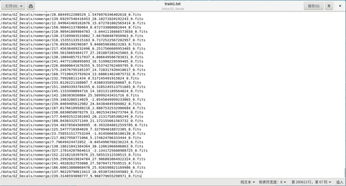
*In the first step, we first filter out the galaxy data with data shape [3*256*256], and save the galaxy data paths that match this shape into a text file, which constitutes our training set. As shown in the example of text in the figure below: | *In the first step, we first filter out the galaxy data with data shape [3*256*256], and save the galaxy data paths that match this shape into a text file, which constitutes our training set. As shown in the example of text in the figure below: | ||
*From more than 300,000 data, 290613 galaxies data matching the shape conditions were selected. | |||
*From more than | |||
== | ==VAE Method== | ||
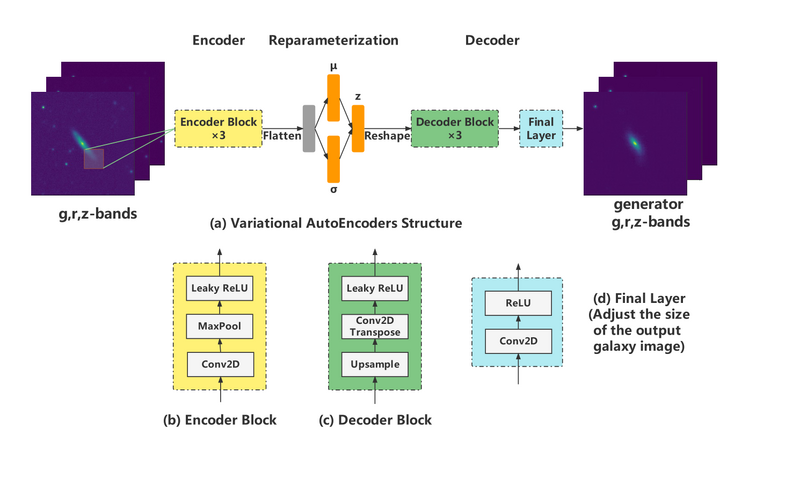
*The neural network of VAE structure is constructed as follows: | |||
[[File:VAE_NN.png|800px|center|jumengting]] | |||
*The neural network structure | |||
[[File: | |||
==Result== | ==Result== | ||
=== | ===Latent variable dimensional analysis=== | ||
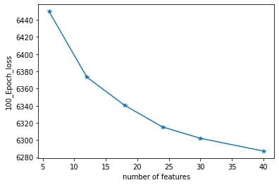
*The | *The number of latent space dimensions is set, and the neural network is used to perform gradient descent fitting to the appropriate case and observe the losses. The following figure represents the losses of different latent space dimensions corresponding to training 100 epochs: | ||
[[File: | [[File:下载11.png|500px|center|jumengting]] | ||
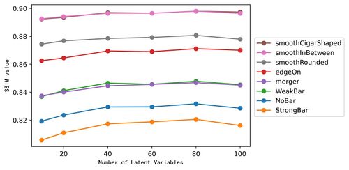
=== | *Evaluation of different latent variable dimensions in various categories of SSIM reconstructed values. | ||
* | [[File:Ssim num1.jpg|500px|center|jumengting]] | ||
=== | *The above are the different representations in different latent spaces. | ||
* | *The higher the dimensionality of the latent variable, the more information in the high-dimensional space it can represent, and the better the quality of the reconstructed image. | ||
*Therefore, considering the dimensionality of the latent variable and the quality of the reconstructed images in a balanced way, the experimental results with loss function of MSE and latent variable features in forty dimensions are selected for further analysis in this work. | |||
*The above is the first stage. | |||
===Latent variables and galaxy morphology=== | |||
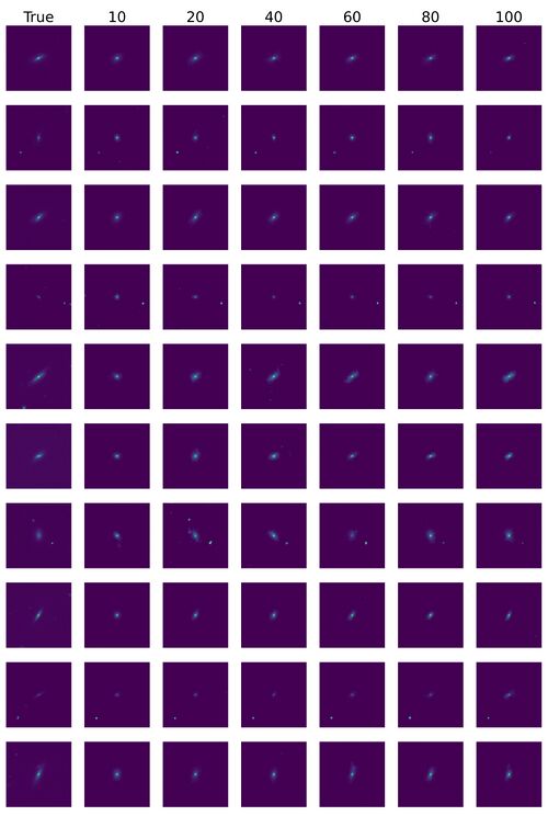
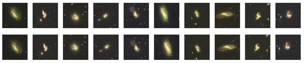
*Some reconstructed images. | |||
[[File:Xiang1.jpg|500px|center|jumengting]] | |||
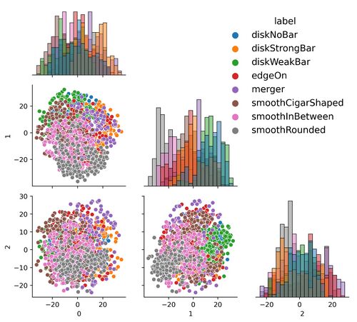
*Latent Space Analysis. | |||
[[File:All.jpg|500px|center|jumengting]] | |||
*The effect of using random forest to classify hidden variables is good. The details will be published in the paper. | |||
===Outlier Latent Variable=== | |||
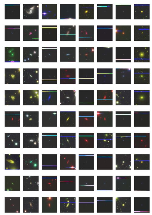
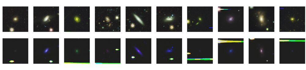
*We find 1308 outliers, accounting for 0.417% of the overall galaxy image. | |||
[[File:Xiyou (1).jpg|500px|center|jumengting]] | |||
*The outliers of the latent variable space are extracted to find rare morphological feature galaxy images and anomalous galaxy images. | |||
== | ==Domain Adaptation== | ||
===Data=== | |||
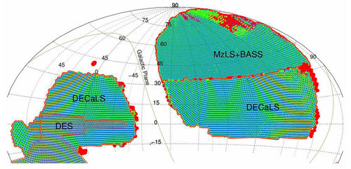
* In this work, we take two different surveys in DESI as an example of transfer between DECaLS and BASS+MaLS overlapping sky region data. | |||
[[File:Fig2.png|500px|center|jumengting]] | |||
===Question=== | |||
* Apply VAE to DECaLS and non-DECaLS to view the latent variable distance. | |||
* Like. | |||
[[File:In out like.jpg|1000px|center|jumengting]] | |||
* DisLike. | |||
[[File:In out dislike.jpg|1000px|center|jumengting]] | |||
===Methods=== | |||
*The Transfer Learning Model of VAE: | |||
===Results=== | |||
See in [https://doi.org/10.1093/mnras/stad3181 paper] | |||
The address of the data is as follows: http://202.127.29.3/~shen/VAE/ | |||
Latest revision as of 18:47, 24 November 2023
Introduction
- This work is divided into two parts.
- The first part is to reduce the dimension of Galaxy data to low dimensional space with VAE.

Datasets
- DECaLS
- In the first step, we first filter out the galaxy data with data shape [3*256*256], and save the galaxy data paths that match this shape into a text file, which constitutes our training set. As shown in the example of text in the figure below:
- From more than 300,000 data, 290613 galaxies data matching the shape conditions were selected.
VAE Method
- The neural network of VAE structure is constructed as follows:

Result
Latent variable dimensional analysis
- The number of latent space dimensions is set, and the neural network is used to perform gradient descent fitting to the appropriate case and observe the losses. The following figure represents the losses of different latent space dimensions corresponding to training 100 epochs:

- Evaluation of different latent variable dimensions in various categories of SSIM reconstructed values.

- The above are the different representations in different latent spaces.
- The higher the dimensionality of the latent variable, the more information in the high-dimensional space it can represent, and the better the quality of the reconstructed image.
- Therefore, considering the dimensionality of the latent variable and the quality of the reconstructed images in a balanced way, the experimental results with loss function of MSE and latent variable features in forty dimensions are selected for further analysis in this work.
- The above is the first stage.
Latent variables and galaxy morphology
- Some reconstructed images.

- Latent Space Analysis.

- The effect of using random forest to classify hidden variables is good. The details will be published in the paper.
Outlier Latent Variable
- We find 1308 outliers, accounting for 0.417% of the overall galaxy image.
.jpg)
- The outliers of the latent variable space are extracted to find rare morphological feature galaxy images and anomalous galaxy images.
Domain Adaptation
Data
- In this work, we take two different surveys in DESI as an example of transfer between DECaLS and BASS+MaLS overlapping sky region data.

Question
- Apply VAE to DECaLS and non-DECaLS to view the latent variable distance.
- Like.

- DisLike.

Methods
- The Transfer Learning Model of VAE:
Results
See in paper
The address of the data is as follows: http://202.127.29.3/~shen/VAE/