Auto clustering of galaxies after dimensionality reduction

Introduction

• This work is divided into two parts.
• The first part is to reduce the dimension of Galaxy data to low dimensional space with VAE.

Datasets

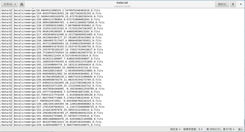
• In the first step, we first filter out the galaxy data with data shape [3*256*256], and save the galaxy data paths that match this shape into a text file, which constitutes our training set. As shown in the example of text in the figure below:

• From more than 300，000 data, 290613 galaxies data matching the shape conditions were selected.

Generate Method

First Method

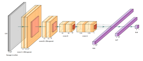
• The neural network structure used in the experiments to construct a neural network structure similar to the original text is shown in the following figure.
• Firstly, GalSim is used to generate information files of relevant galaxies based on random parameters. Because deep learning requires a large number of images and parameter samples, the cost of manual annotation of images is too high; and the expertise of the person conducting the annotation is required. Generating datasets with parameters is a more convenient experimental method.
• When generating galaxy data with GalSim software, the dimension size of the generated data is also set to random because the dimension size of the real galaxy data varies. The python library is used to generate 50,000 galaxy information, which is partitioned into a training set, a test set, and a validation set in the ratio of 8:1:1. In order to handle galaxy images of different sizes, this paper uses two-dimensional data with a standard size of 128*128 size, which will be different in shape from 128*128 size, cut the center of galaxy images larger than 128*128 pixels, and fill the edges of images smaller than 128*128 pixels.

Second NN

• The second task fits the data to multiple parameters.

Result

Generate data First Method

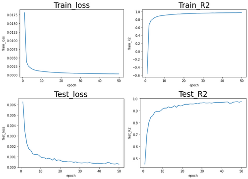
• The above network fits the galaxy data to one parameter using a 2D convolutional neural network. The following are the training results for training a single parameter - star magnitude.

Generate data Second Method

• Galsim result.

Ground-Truth data Second Method

• CANDELS

Else

Waiting...

 (II) The neural network of VAE structure is constructed as follows:
VAE(
 (encoder): Sequential(
   (0): Sequential(
     (0): Conv2d(3, 32, kernel_size=(3, 3), stride=(2, 2), padding=(1, 1))
     (1): BatchNorm2d(32, eps=1e-05, momentum=0.1, affine=True, track_running_stats=True)
     (2): LeakyReLU(negative_slope=0.01)
   )
   (1): Sequential(
     (0): Conv2d(32, 64, kernel_size=(3, 3), stride=(2, 2), padding=(1, 1))
     (1): BatchNorm2d(64, eps=1e-05, momentum=0.1, affine=True, track_running_stats=True)
     (2): LeakyReLU(negative_slope=0.01)
   )
   (2): Sequential(
     (0): Conv2d(64, 128, kernel_size=(3, 3), stride=(2, 2), padding=(1, 1))
     (1): BatchNorm2d(128, eps=1e-05, momentum=0.1, affine=True, track_running_stats=True)
     (2): LeakyReLU(negative_slope=0.01)
   )
   (3): Sequential(
     (0): Conv2d(128, 256, kernel_size=(3, 3), stride=(2, 2), padding=(1, 1))
     (1): BatchNorm2d(256, eps=1e-05, momentum=0.1, affine=True, track_running_stats=True)
     (2): LeakyReLU(negative_slope=0.01)
   )
   (4): Sequential(
     (0): Conv2d(256, 512, kernel_size=(3, 3), stride=(2, 2), padding=(1, 1))
     (1): BatchNorm2d(512, eps=1e-05, momentum=0.1, affine=True, track_running_stats=True)
     (2): LeakyReLU(negative_slope=0.01)
   )
 )
 (fc_mu): Linear(in_features=32768, out_features=35, bias=True)
 (fc_var): Linear(in_features=32768, out_features=35, bias=True)
 (decoder_input): Linear(in_features=35, out_features=32768, bias=True)
 (decoder): Sequential(
   (0): Sequential(
     (0): ConvTranspose2d(512, 256, kernel_size=(3, 3), stride=(2, 2), padding=(1, 1), output_padding=(1, 1))
     (1): BatchNorm2d(256, eps=1e-05, momentum=0.1, affine=True, track_running_stats=True)
     (2): LeakyReLU(negative_slope=0.01)
   )
   (1): Sequential(
     (0): ConvTranspose2d(256, 128, kernel_size=(3, 3), stride=(2, 2), padding=(1, 1), output_padding=(1, 1))
     (1): BatchNorm2d(128, eps=1e-05, momentum=0.1, affine=True, track_running_stats=True)
     (2): LeakyReLU(negative_slope=0.01)
   )
   (2): Sequential(
     (0): ConvTranspose2d(128, 64, kernel_size=(3, 3), stride=(2, 2), padding=(1, 1), output_padding=(1, 1))
     (1): BatchNorm2d(64, eps=1e-05, momentum=0.1, affine=True, track_running_stats=True)
     (2): LeakyReLU(negative_slope=0.01)
   )
   (3): Sequential(
     (0): ConvTranspose2d(64, 32, kernel_size=(3, 3), stride=(2, 2), padding=(1, 1), output_padding=(1, 1))
     (1): BatchNorm2d(32, eps=1e-05, momentum=0.1, affine=True, track_running_stats=True)
     (2): LeakyReLU(negative_slope=0.01)
   )
 )
 (final_layer): Sequential(
   (0): ConvTranspose2d(32, 32, kernel_size=(3, 3), stride=(2, 2), padding=(1, 1), output_padding=(1, 1))
   (1): BatchNorm2d(32, eps=1e-05, momentum=0.1, affine=True, track_running_stats=True)
   (2): LeakyReLU(negative_slope=0.01)
   (3): Conv2d(32, 3, kernel_size=(3, 3), stride=(1, 1), padding=(1, 1))
   (4): Tanh()
 )
)
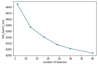
 (III) The number of latent space dimensions is set, and the neural network is used to perform gradient descent fitting to the appropriate case and observe the losses. The following figure represents the losses of different latent space dimensions corresponding to training 100 epochs:

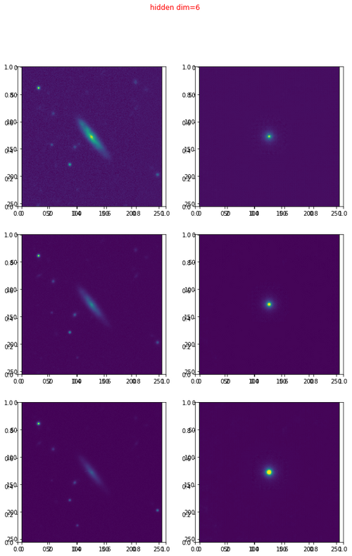
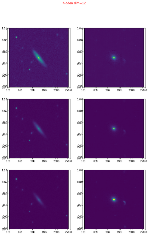
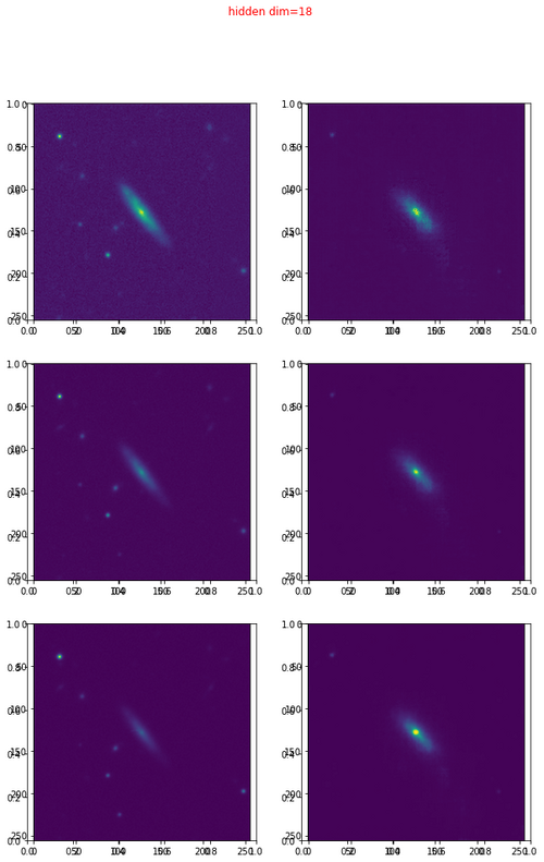
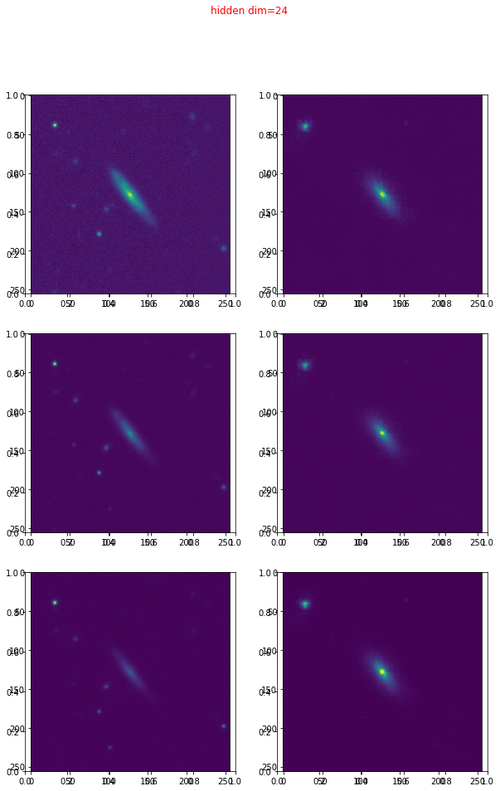
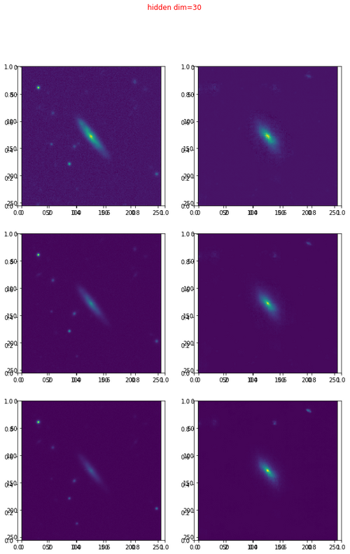
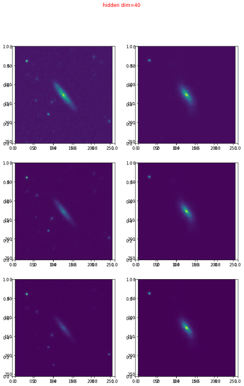
 The following are the different representations in different latent spaces:

 The higher the dimensionality of the latent variable, the more information in the high-dimensional space it can represent, and the better the quality of the reconstructed image.
 The above is the first stage.
 The address of the data is as follows: http://202.127.29.3/~shen/VAE/