Auto clustering of galaxies after dimensionality reduction

 This work is divided into two parts.
 The first part is to reduce the dimension of Galaxy data to low dimensional space with VAE.
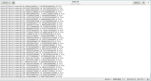
 (I) In the first step, we first filter out the galaxy data with data shape [3*256*256], and save the galaxy data paths that match this shape into a text file, which constitutes our training set. As shown in the example of text in the figure below:

 From more than 300，000 data, 290613 galaxies data matching the shape conditions were selected.
 (II) The neural network of VAE structure is constructed as follows:
VAE(
 (encoder): Sequential(
   (0): Sequential(
     (0): Conv2d(3, 32, kernel_size=(3, 3), stride=(2, 2), padding=(1, 1))
     (1): BatchNorm2d(32, eps=1e-05, momentum=0.1, affine=True, track_running_stats=True)
     (2): LeakyReLU(negative_slope=0.01)
   )
   (1): Sequential(
     (0): Conv2d(32, 64, kernel_size=(3, 3), stride=(2, 2), padding=(1, 1))
     (1): BatchNorm2d(64, eps=1e-05, momentum=0.1, affine=True, track_running_stats=True)
     (2): LeakyReLU(negative_slope=0.01)
   )
   (2): Sequential(
     (0): Conv2d(64, 128, kernel_size=(3, 3), stride=(2, 2), padding=(1, 1))
     (1): BatchNorm2d(128, eps=1e-05, momentum=0.1, affine=True, track_running_stats=True)
     (2): LeakyReLU(negative_slope=0.01)
   )
   (3): Sequential(
     (0): Conv2d(128, 256, kernel_size=(3, 3), stride=(2, 2), padding=(1, 1))
     (1): BatchNorm2d(256, eps=1e-05, momentum=0.1, affine=True, track_running_stats=True)
     (2): LeakyReLU(negative_slope=0.01)
   )
   (4): Sequential(
     (0): Conv2d(256, 512, kernel_size=(3, 3), stride=(2, 2), padding=(1, 1))
     (1): BatchNorm2d(512, eps=1e-05, momentum=0.1, affine=True, track_running_stats=True)
     (2): LeakyReLU(negative_slope=0.01)
   )
 )
 (fc_mu): Linear(in_features=32768, out_features=35, bias=True)
 (fc_var): Linear(in_features=32768, out_features=35, bias=True)
 (decoder_input): Linear(in_features=35, out_features=32768, bias=True)
 (decoder): Sequential(
   (0): Sequential(
     (0): ConvTranspose2d(512, 256, kernel_size=(3, 3), stride=(2, 2), padding=(1, 1), output_padding=(1, 1))
     (1): BatchNorm2d(256, eps=1e-05, momentum=0.1, affine=True, track_running_stats=True)
     (2): LeakyReLU(negative_slope=0.01)
   )
   (1): Sequential(
     (0): ConvTranspose2d(256, 128, kernel_size=(3, 3), stride=(2, 2), padding=(1, 1), output_padding=(1, 1))
     (1): BatchNorm2d(128, eps=1e-05, momentum=0.1, affine=True, track_running_stats=True)
     (2): LeakyReLU(negative_slope=0.01)
   )
   (2): Sequential(
     (0): ConvTranspose2d(128, 64, kernel_size=(3, 3), stride=(2, 2), padding=(1, 1), output_padding=(1, 1))
     (1): BatchNorm2d(64, eps=1e-05, momentum=0.1, affine=True, track_running_stats=True)
     (2): LeakyReLU(negative_slope=0.01)
   )
   (3): Sequential(
     (0): ConvTranspose2d(64, 32, kernel_size=(3, 3), stride=(2, 2), padding=(1, 1), output_padding=(1, 1))
     (1): BatchNorm2d(32, eps=1e-05, momentum=0.1, affine=True, track_running_stats=True)
     (2): LeakyReLU(negative_slope=0.01)
   )
 )
 (final_layer): Sequential(
   (0): ConvTranspose2d(32, 32, kernel_size=(3, 3), stride=(2, 2), padding=(1, 1), output_padding=(1, 1))
   (1): BatchNorm2d(32, eps=1e-05, momentum=0.1, affine=True, track_running_stats=True)
   (2): LeakyReLU(negative_slope=0.01)
   (3): Conv2d(32, 3, kernel_size=(3, 3), stride=(1, 1), padding=(1, 1))
   (4): Tanh()
 )
)
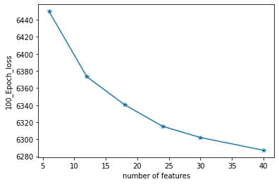
 (III) The number of latent space dimensions is set, and the neural network is used to perform gradient descent fitting to the appropriate case and observe the losses. The following figure represents the losses of different latent space dimensions corresponding to training 100 epochs:

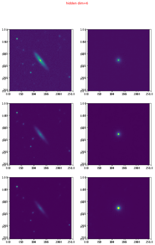
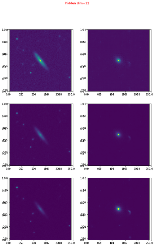
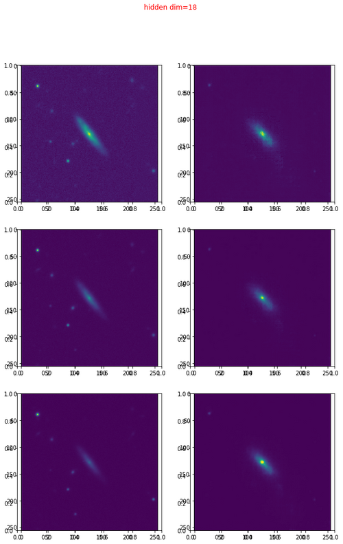
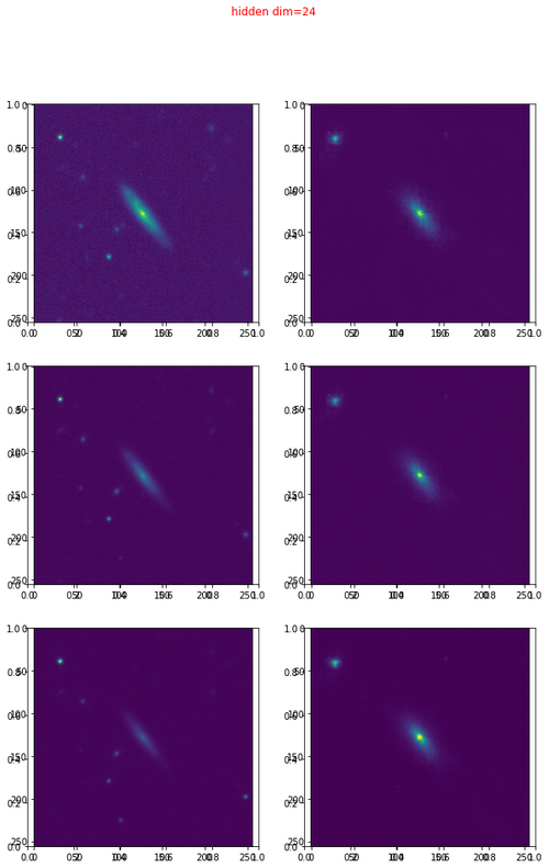
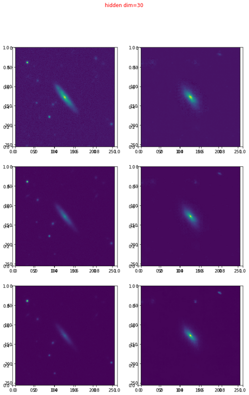
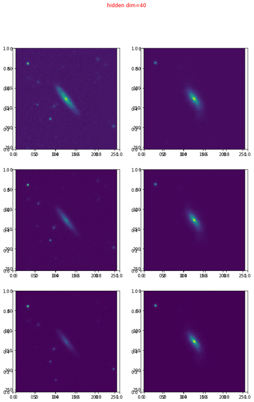
 The following are the different representations in different latent spaces:

文件:X129.png